Reading Binding Characterization Results

A binding experiment answers three questions about every design you send us: does it bind the target, how tightly, and how fast it comes off. A characterization run resolves each interaction into three numbers (kon, koff, and KD) from a family of sensorgrams measured across a concentration series. This guide is the field manual for that output: how the assay produces the curve, what the curve is telling you, and how much to trust the fitted numbers. It sits alongside the Binding experiment overview and the Binding Data Package reference, which documents every file in your download.

How the assay works

We measure binding with biolayer interferometry (BLI) on a Gator Bio Pro, and surface plasmon resonance (SPR) on a Carterra LSA XT. Both are label-free (nothing is attached to the target to make it visible) and both produce the same readout. We pick the platform that fits the campaign, leaning on SPR as the higher-throughput option for larger sample sets and BLI for smaller ones.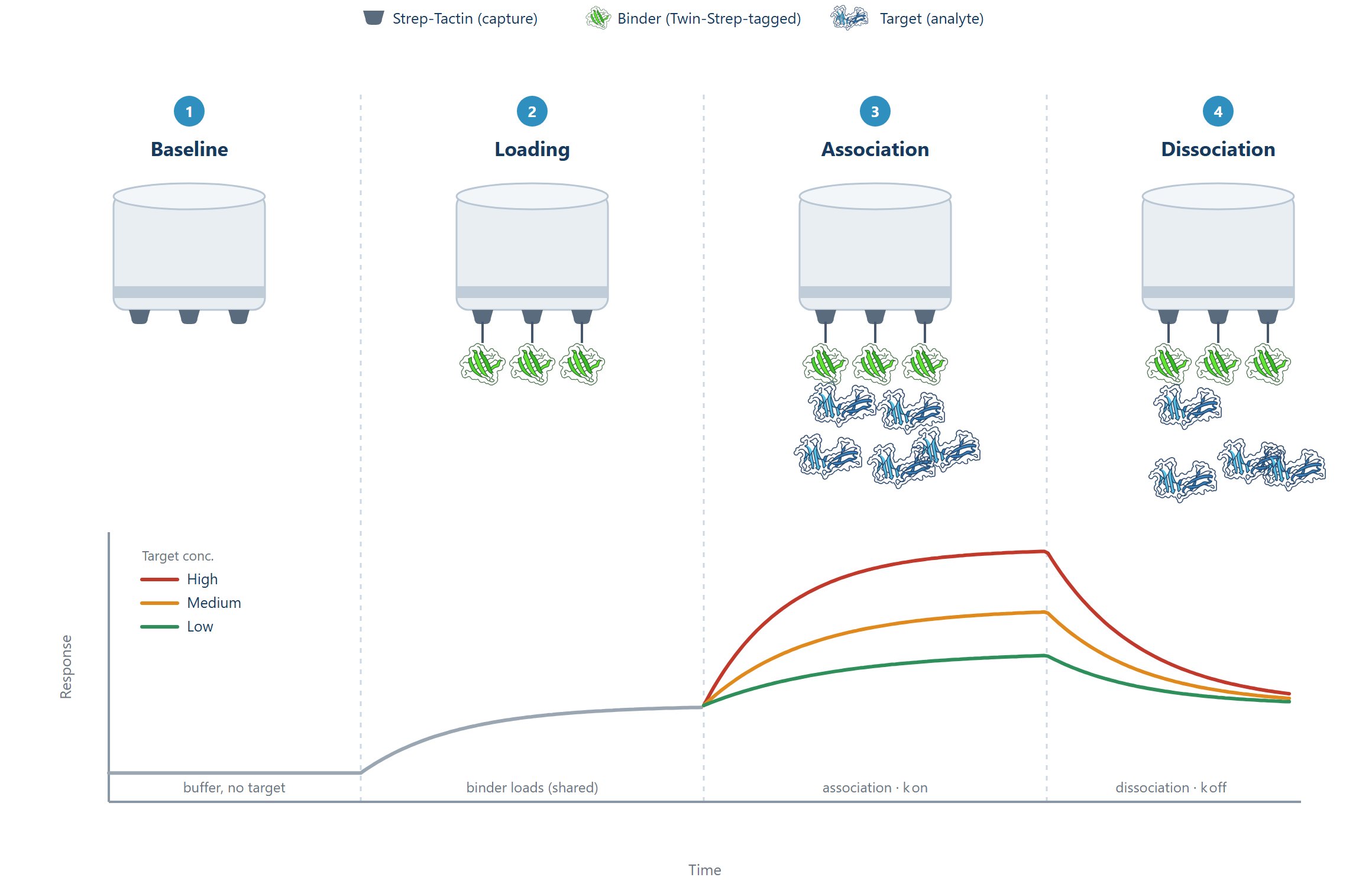

BLI binding assay workflow across four phases: baseline; loading, where a Twin-Strep-tagged binder is captured on the Strep-Tactin surface; association, where target binds; and dissociation. A sensorgram below tracks binding over time, with high, medium, and low target-concentration traces that share one baseline and loading level and diverge only during association. — How a BLI binding run works: the Twin-Strep-tagged binder is captured on the Strep-Tactin biosensor (loading), the target flows over and binds (association), then washes off in buffer (dissociation). The trace tracks binding over time at three target concentrations; association gives kon and dissociation gives koff.

Your protein goes on the sensor

We express each design with a two domain C-terminal tag: a split-GFP fragment (for expression quantification), followed by a Twin-Strep-Tag that anchors it to the biosensor surface facing outward. The full C-terminal tag is RDHMVLHEYVNAAGITGGGSGGGSGGSAWSHPQFEKGGGSGGGSGGSAWSHPQFEK, and your protein is the ligand.

The target flows over it

The sensor is exposed to the target protein (the analyte) at known concentrations. If your design recognizes the target, the two associate at the surface.

We watch binding in real time

Bound target adds mass at the surface, which shifts the optical signal. We record that shift continuously, with no endpoint and no wash-and-read.

Then we let it fall off

Switching exposure to just the buffer solution lets bound target dissociate. The climb and the decay together form the binding curve.

Anatomy of a sensorgram

A sensorgram plots response (mass bound at the sensor surface, in nm for BLI or RU for SPR) against time. One characterization run overlays several curves, one per target concentration, fitted together as a single family.

Annotated sensorgram with three phases: a flat baseline, an association phase where four target concentrations plus a zero-concentration blank rise to concentration-dependent plateaus, and a dissociation phase where every curve decays at the same rate without crossing. The kon and koff phases are labelled. — Reading a sensorgram: an illustrative characterization run, simulated for a KD of 100 nM across the four target concentrations we run plus a zero-concentration blank. Higher concentrations (darker) climb faster and plateau higher during association. During dissociation every curve decays at the same rate, because koff does not depend on concentration; only the height each one starts from differs. Fitting the whole family at once is what pins down the kinetics.

Read each curve left to right in four phases:

Baseline. Sensor in buffer, no target. This is your zero.
Association. Target (“analyte”) is flowing on. Response climbs as target binds your surface-anchored protein (“ligand”). Higher concentrations climb faster and toward a higher plateau.
Approach to steady state. The climb curves over as binding and unbinding reach balance. Whether a curve actually reaches its plateau depends on concentration, kon, and how long the injection runs.
Dissociation. Flow switches to buffer only. No fresh target arrives, so bound target falls off and the response decays.

The information lives in the shape, not the height. The steepness of the climb encodes kon, the steepness of the decay encodes koff, and the concentration-dependent spacing between curves is what lets a global fit separate the two. A single concentration can’t. That’s why characterization runs a series rather than one point: four concentrations spanning roughly a hundred-fold range, plus a zero-concentration blank.koff is the one thing that does not change with concentration. Every curve in a family should fall away at the same rate during dissociation, starting from whatever height it reached. Curves that decay at visibly different rates, or that cross during dissociation, are a sign the interaction isn’t a simple 1:1.

The three numbers

Every characterization fit reports the same three values, each with a 95% confidence interval.

Value	What it is	Where it comes from
`kon`	Association rate (M⁻¹s⁻¹): how fast target finds and binds	Steepness of the association climb, across concentrations
`koff`	Dissociation rate (s⁻¹): how fast it lets go	Steepness of the dissociation decay
`KD`	Affinity (M) = `koff` / `kon`, the concentration at which half your protein is occupied	Derived from the two rates

Lower KD is tighter: a 1 nM binder is 1000× stronger than a 1 µM one. But two designs can reach the same KD by opposite routes (one fast-on/fast-off, the other slow-on/slow-off), and they often behave differently in your application. A slow koff (long residence time) is frequently what matters most. That’s why we report the rates, not just the affinity.

koff is usually the more decision-relevant rate. Read it directly off the dissociation phase: a curve that barely comes down has a slow koff and a long residence time, regardless of how fast it went on.

Screening and characterization

The difference between the two is simply how many concentrations we run, and that determines whether you get a ranking or a real number. Most campaigns do both: screen the library wide, then characterize the handful of winners.

	Binding screening	Affinity characterization
Concentrations	2, plus a zero-concentration blank	4, plus a zero-concentration blank
You get	Strong / Moderate / Weak / Non-binder, with ranked responses	Quantitative `KD`, `kon`, `koff` with confidence intervals and fit diagnostics
`KD` precision	Indicative bucket	Quantitative, ≈ 0.1 nM–10 µM
Best for	Triaging large libraries, down-selection	Lead optimization, benchmarking, mechanism studies
The question	Which of my designs bind?	Exactly how good is my best one?

Why the extra concentrations matter: a single point can be explained by many curves, but a series spanning several concentrations constrains the fit and lets us separate kon from koff. That’s why a characterization KD is trustworthy where a screening estimate is only indicative.

Reading your results

Every measured design gets a binding call. How its strength is reported then depends on the depth you ran: a quick bucket from screening, or precise kinetics from characterization.

Did it bind?

Call	What it means
True	A clear binder: signal rises distinctly above the controls.
False	The protein expressed, but binding sits at or below control signals. No interaction detected.
Unknown	We couldn’t make the call, usually because of no/low expression or signals too marginal to trust.

How strong? From a screening run

Screening sorts each binder into one of three affinity buckets, enough to rank a library and decide what to pursue.

Bucket	Range
Strong	`KD` < 50 nM
Moderate	50 nM–1 µM
Weak	> 1 µM

How strong? From a characterization run

A full concentration series resolves the interaction into quantitative kinetics, each reported with a 95% confidence interval, alongside fit-quality diagnostics so you can judge how much to trust the numbers.

	Value	95% CI
`KD`	4.2 nM	3.6–4.9 nM
`kon`	2.1 × 10⁵ M⁻¹s⁻¹	1.9–2.3 × 10⁵
`koff`	8.9 × 10⁻⁴ s⁻¹	8.1–9.6 × 10⁻⁴

Each value comes from the global fit across the whole series; the confidence interval shows how tightly that fit is constrained, and the diagnostics (below) flag any curve worth a closer look.

Binding depends on expression. We can only measure binding for protein that actually made it onto the sensor. A poorly-expressed design gives low signal-to-noise, wide CIs, and often an Unknown call rather than a KD. Confirming expression first is the surest route to clean, tightly-fitted curves.

Judging fit quality

The fitted numbers are only as good as the fit they came from. Every characterization result ships with diagnostics, both in the portal and in the fit_data/ folder of your data package, so you can judge each one yourself. Four things to check:

Confidence intervals. Each rate carries a 95% CI. Tight, symmetric intervals (a few percent of the value) mean the fit is well-constrained. A CI that spans an order of magnitude means the data don’t pin that parameter down, so treat the number as indicative, not quantitative.
Fit error (MAE). The mean absolute error between the modelled and measured curves, reported per replicate. Low MAE relative to the signal is good. The stronger test is the residuals: plot model-minus-data and you want flat, random noise around zero. Systematic structure, like a bowed or S-shaped residual, means the model isn’t capturing what the surface actually did.
Rmax. The estimated maximum response, i.e. a fully-loaded surface. A physically sensible Rmax should agree with the theoretical Rmax the surface can support: Rmax(theoretical) = (analyte MW / ligand MW) × immobilized ligand level × binding sites per ligand. In practice the measured Rmax usually lands around 30–70% of that value. A measured Rmax far below theoretical (a few percent of predicted, in the worst cases) points to a misfolded or aggregating surface; an Rmax above theoretical points to non-specific binding, analyte aggregation, or an association phase that never curved enough to constrain the fit.
Range. We reliably quantify KD from roughly 0.1 nM to 10 µM. Outside that window a value may be reported as a bound (see below) rather than a point estimate.

Common curve shapes

Most designs give a clean 1:1 curve. When they don’t, the shape tells you why, and whether the fitted KD still means what you think. Use this as a lookup.

Ideal 1:1 (Langmuir). Smooth exponential rise to a clear plateau during association; smooth single-exponential decay at the same rate for every curve during dissociation. Curves fan out by concentration, and the highest concentrations flatten at the same height because they have saturated the surface (Rmax). Residuals are flat noise. Trust the numbers: this is the case the fit is built for.

Never reaches plateau. Association is still climbing when the injection ends, with no curvature. Either kon is slow or every concentration sits below KD. The fit can still work if dissociation is well-defined, but KD leans on extrapolation; widen the concentration range to tighten it.Suggestion. Add higher concentrations, or extend the association time, so the curves approach saturation and pin down KD.

Flat dissociation (no come-off). The decay barely drops within the dissociation window. The target essentially doesn’t let go. koff is slower than the experiment can measure, so it (and therefore KD) is reported as an upper bound: ”≤” a value, not ”=”. Typical of very tight binders. Longer dissociation times can pull it into range.Suggestion. Ask for a longer dissociation window (up to 30–60 min) so koff can be resolved; otherwise KD stays an upper bound.

Fast-on / fast-off (square wave). Rapid rise, low plateau, rapid return to baseline the instant buffer flows. A weak, fast-equilibrating interaction where the kinetics are too fast to resolve. Here steady-state (equilibrium) analysis (response at plateau vs. concentration) gives a more reliable KD than the kinetic fit.Suggestion. Use steady-state (equilibrium) analysis, and widen the concentration range so it brackets KD.

Mass-transport limitation. Association looks oddly linear instead of exponential because target is binding faster than flow can replenish it at the surface. This underestimates kon. Diagnostic: apparent kon changes with flow rate. We mitigate it with lower ligand density and higher flow; if it persists we flag the affected fits.Suggestion. Lower the ligand density and raise the flow rate, then confirm kon no longer changes with flow.

Biphasic / heterogeneous. Two visibly different phases: a fast then a slow component in the association or (more often) the dissociation. Points to avidity, a heterogeneous or partly-misfolded ligand population, a conformational change, or aggregation. A 1:1 fit will show systematic residuals; we report these with caveats and, where it helps, an alternative model.Suggestion. Ask for the flipped assay and HPLC-SEC to find the cause (avidity, heterogeneity, or aggregation); we can also fit a bivalent or conformational model, or report ranking-only.

Non-specific binding / drift. Signal keeps drifting upward during dissociation, or the reference channel itself responds. A “sticky” analyte or surface inflates apparent binding. Reference and blank (buffer) subtraction remove most of it; a curve that survives subtraction is real.Suggestion. Improve reference and blank subtraction, adjust the buffer or blocking, or lower the analyte concentration; a curve that survives subtraction is real.

Super-stoichiometric (aggregation). Response climbs past a sensible Rmax without saturating, because more mass lands than a monolayer of target should allow, usually from analyte self-association at the surface. The KD from a 1:1 fit is unreliable; cleaner material or lower concentrations are the fix.Suggestion. Re-run with cleaner, monomeric material (SEC-purified) at lower concentrations, and use a dilution series to confirm; the 1:1 KD here is not reliable.

Before quoting a KD, glance at the sensorgram PNG in your data package and match it to one of the shapes above. Ninety seconds of eyeballing catches the cases where a number is technically fitted but not trustworthy.

When the curve isn’t 1:1

When a curve doesn’t fit a clean 1:1 model, the two most common reasons are avidity and aggregation, and each changes what the KD actually means. We fit a 1:1 model first; when the shape rejects it, we fit alternative models (bivalent, conformational), and when a curve can’t be trusted at all we report the binder as a ranked hit without a KD rather than quote a number we don’t believe.

Apparent KD and avidity

Binding curves are fit assuming a 1:1 interaction. Some systems show avidity, where a binder or a multivalent target engages more than one site at once. Avidity slows dissociation, so the interaction looks stronger than it is, and the reported KD is an apparent KD, not a true thermodynamic constant. This is common when the target is oligomeric (dimeric, trimeric, or Fc-tagged): the observed koff is artificially slow and the KD artificially tight. Avidity can be a deliberate design feature (a bispecific engaging two epitopes on the same target can dissociate several-fold more slowly by design) or an artifact of how the protein sits on the surface. Because of this, the platform is tuned to rank binders consistently rather than to report absolute biophysical constants.

To separate true affinity from surface avidity, ask us for a flipped assay: we put the target on the sensor and titrate your binder in solution. A genuine 1:1 interaction gives a clean fit; a shape that only looked tight because of avidity resolves.

Aggregation

A misfolded or aggregating construct can produce a signal that reads tight but isn’t real binding. The tells are consistent: unusually high loading for the protein’s size, a response well below the expected Rmax, very slow association and dissociation, and a sensorgram that won’t fit a clean 1:1 (often resembling non-specific binding). We flag these and confirm them with orthogonal checks: a dilution series (real binding tracks loading, aggregation doesn’t), the flipped assay above, an extended dissociation window, and HPLC-SEC to see aggregation directly. When aggregation is confirmed, the KD isn’t reliable, so we revise or withhold it rather than report it.

Both platforms can agree and still be wrong. In one revalidation, aggregating binders reproduced the same false-positive signal on both SPR and BLI; it took the flipped assay and HPLC-SEC to catch it. When a number looks too good, the check is the biophysics (loading, Rmax, curve shape), not just the goodness of fit.

What you get back

Beyond the summary call and kinetic values in the portal, every binding experiment comes with a downloadable data package: the underlying traces, fits, and QC, ready for your own analysis. Everything in it is safe to share and pipeline-friendly.

File	What it is
Sensorgrams	A binding-curve PNG for every sample and replicate, for quick visual QC without touching the raw data.
Raw traces (`.csv`)	Instrument readouts as time vs. response in nanometers, one file per concentration.
Fitted curves	The modelled sensorgrams for approved fits; overlay them on the raw traces to reproduce the kinetics.
Per-replicate QC	Fit error (MAE), method, and estimated `Rmax` so you can judge each fit yourself.

FAQs

Why don't I always get a KD?

A KD requires enough of your protein on the sensor to give clean signal. If expression is none or low, signal-to-noise is too poor for a reliable fit, so the result comes back as Unknown rather than a number. Stronger expression yields cleaner curves and tighter fits.

What KD range can you quantify?

Roughly 0.1 nM to 10 µM. Accuracy tapers at the extremes (very tight or very weak interactions are harder to pin down), but we can tune concentrations and contact times to bias the assay toward either end when you know what you’re chasing.

How are the curves fitted?

We record response over time at 5 Hz and fit a 1:1 binding model. When several concentrations are run, we fit them together (global fitting) so a single kon/koff pair has to explain the whole family of curves, a much stronger constraint than fitting one trace alone.

Why do screening KDs differ from full characterization?

Screening uses only two concentrations to triage binders quickly, so its KD carries more uncertainty. Characterization runs a full series designed to resolve kon, koff, and KD precisely. Treat screening values as a ranking, not a measurement.

What about unusual or bi-phasic curves?

Curves that don’t fit a clean 1:1 model can point to a multi-step mechanism, conformational change, or avidity. Relative rankings still hold, but resolving precise kinetics may need an expanded concentration series. We’ll flag these when we see them.

How do you handle non-specific binding?

We screen new targets for non-specific binding (NSB) and adjust buffers or suppliers to suppress it. Heavy NSB can show up as negative-shift curves after reference subtraction, a tell we watch for during QC.

Can you test specificity and cross-reactivity?

Yes. We run cross-reactivity and polyspecificity panels (e.g. BVP, BSA/HSA) to check how selective your binder is. Full-serum profiling is in development.

Do you offer competition or inhibition assays?

Yes. We run neutralization, inhibition, and competition formats (IC50 and epitope-access questions) on request.

Ready to run a binding experiment? Configure your target, upload sequences, and get a quote in minutes at start.adaptyvbio.com/binding.

Binding experiment overview

What the assay measures, and screening vs. characterization.

Binding Data Package

Every folder and file in your download, including the fit diagnostics referenced here.

Improve Protein Expression

Clean binding data starts with protein that expresses well.

Guides

Protein Design 101

Reading Binding Characterization Results

How the assay works

Anatomy of a sensorgram

The three numbers

Screening and characterization